CSE 455 Depth Perception Project
Abstract
Theory
In order to deduce depth perception we are in need of 2 cameras at a specified horizontal distance to each other and are relatively on the same vertical axis. Both cameras are required to take pictures at the same time of the same scene in order to deduce depth. It does so by using Stereo Disparity, which is the difference in image location from the left and right image taken from the camera.
The rationale provided above is also the reason why a single camera is not sufficient to deduce depth, at least without being aided with the help of neural networks or using Active stereo with the employment of light.
In order to use the Disparity to deduce depth we have to then use Triangulation which is a geometric approach used to deduce depth.
In order to go about this math we must understand that there are 3 planes we travel in between in order to deduce depth. There is the world coordinate plane, the camera coordinate plane and the image coordinate plane. Image plane is where the image sensor lies and the camera plane is where the lens lies. A transformation is undergone from 3D to 2D when we tranform the coordinates from the world coordinates to the image coordinates and vice versa. The transformation from the world coordinates to the camera coordinates is a 3-D to 3-D tranformation and the tranformation from the camera to the image plane in a 3-D to 2-D transformation.
Camera Calibration
Based on our working understanding of perspective projections we can infer the image coordinates with respect to the camera.
Where \(x_{i}\) = image coords in \(x\), \(x_{c}\) = camera coords in \(x\), \(z_{c}\) = camera coords in \(z\), \(f\) = focal length, \(y_{i}\) = image coords in \(y\), \(y_{c}\) = camera coords in \(y\).
Bearing in mind that the image coordinates are captures by the image sensors of the cameras, we need to transform the coordinates once more from standard coordinates to pixels. When doing that we realize that the pixels themselves need not necessarily be square in nature but may also be rectangular.
The principal is with respect to the top left corner of an image.
Where \(m_{x}\) = pixel density in \(x\), \(o_{x}\) = principal point in \(x\). \(m_{y}\) = pixel density in \(y\), \(o_{y}\) = principal point in \(y\).
The directional focal lengths and the principal point is referred to as the camera’s internal geometry, thus bearing out the intrinsic matrix.
Once we gain the 2D parameters of the image we have convert it into its homogenous 3D representation in order to do the transformation into the camera’s coordinate system.
Now we have to do the mapping from camera coordinate frame to the world coordinate frame which is a 3D to 3D transformation, this done knowing the position and orientation of the camera coordinate frame with respect to the world coordinate frame.
It should be noted that the rotation matrix is a orthonormal matrix as in, when a dot product is carried by itself it produces an Identity matrix and its inverse is equivalent to its transpose.
Where \(X_{c}\) is a vector from the camera to any point in world coordinate frame, \(C_{w}\) is a vector from world coordinates to any point.
\[X_{c}=\left[\begin{array}{l} x_{c} \\ y_{c} \\ z_{c} \end{array}\right]=\left[\begin{array}{lll} r_{11} & r_{12} & r_{13} \\ r_{21} & r_{22} & r_{23} \\ r_{31} & r_{32} & r_{33} \end{array}\right]\left[\begin{array}{l} x_{w} \\ y_{w} \\ z_{w} \end{array}\right]+\left[\begin{array}{l} t_{x} \\ t_{y} \\ t_{z} \end{array}\right]\]In order to get a more concise algorithm to solve things, we can transform our current matrix into Homogenous Coordinates.
As noted from above we see that we can extract the extrinsic matrix that contains the parameters of all involved external parameters and construct the extrinsic matrix.
We can now transform the world coordinates to image coordinates with the transformations we have crafted thus far.
Where \(P\) is the projection matrix.
With this we have calibrated our camera.
Triangulation using 2 Cameras
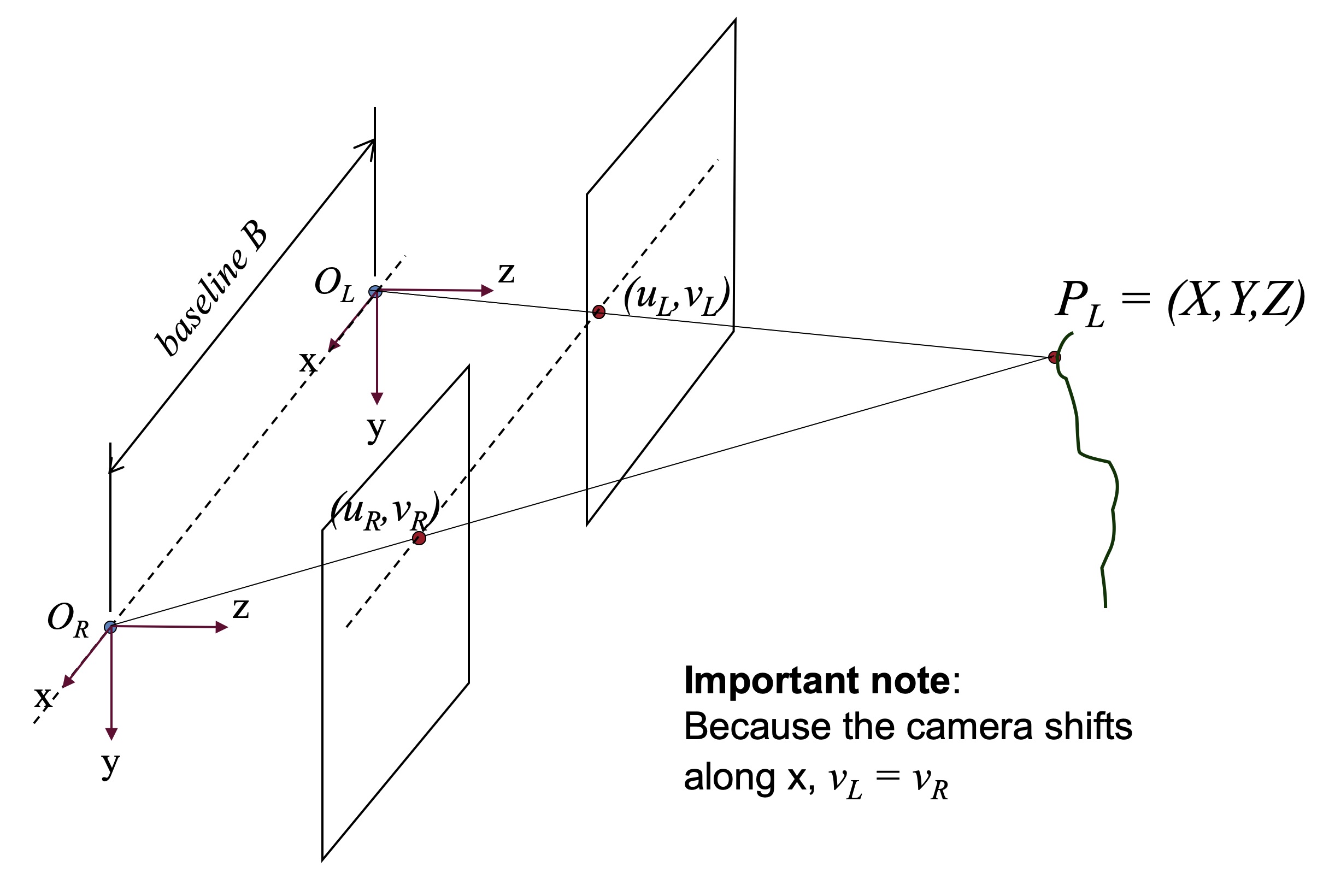
We first have to set up 2 cameras which have been calibrated and are set up apart horizontally by a known distance. There can be no difference in any other aspects of orientation other than the horizontal distance it is set apart by. The kind of stereo vision that is generated is called binocular vision.
The idea is that 2 cameras are seperated by a realtively small horizontal distance. Based on this fact the images captured will be slightly translated relative to one other. So we would need to calibrate both cameras based on earlier but with a single caveat being that the camera that was shifted to the right would have to account for the shift in the horizontal direction.
Where \(b\) is the baseline distance between two lenses.
From the calibration we know of the intrinsic parameters and can re-arrange the equation to find the world coordinates.
Figure one we found online is a good illustration of the provided concepts:
 |
|---|
| Fig. 1. Illustration of triangulation using two cameras. |
Project
The motivation for our project is to create a platform for doing depth perception with two cheap Android phones utilizing stereo vision. There are multiple ways to perceive depth including the use of neural networks however doing it in real time with hardware has many pitfalls which we aim to uncover.
Performing depth perception with readily available hardware (such as old android phones) can be useful for hobbyists, researchers or educationists for integration into larger projects such as localization and mapping with mobile robotics.
The Setup
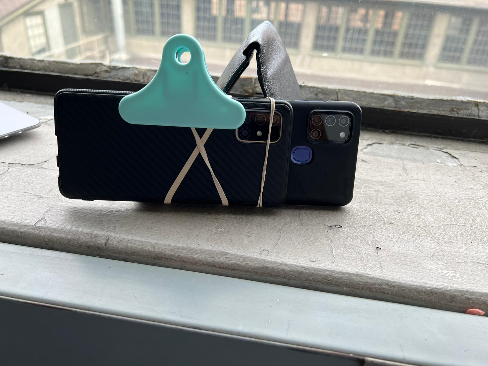
Our setup consisted of two android cameras being used as wireless IP cameras.
 |
|---|
| Fig. 2. Photograph of our stereo camera setup. |
Cameras being used:

We used the application iVcam to stream the video signals from both the cell phones and use the PC client to receive it. We could have directly accessed the phones on the network via openCV however there was a significant lag of as much as ten seconds in the feed.
It is important to note that for a robust real time system to work the video feeds must be synchronized in time, this is impossible as both cameras run on their individual system clocks.
To minimize the delay we used iVcam’s drivers to receive the video and in our code we used cv.grab() and cv.retrieve() to get the two frames and decode them after respectively. The alternative is to use cv.read() which grabs and retrieves together therefore creating the delay of one frame being decoded.
The above measures minimized the delay and iVcam’s client allowed us to tweak the attributes such as exposure, ISO and focus to maintain consistency. The automatic dynamics of the cameras operating individually can create significant problems as the pixel values vary due to lighting and other noises between the two images. In an ideal scenario we want two same images with a fully aligned y axis with only a difference in the x axis to produce disparity.
The best hardware setup is to have the exact same camera setup rigidly connected sharing the same system clock such as the StereoPi.
Here is a simple data collection code you could use to take pictures with your stereo setup:
import numpy as np
import cv2

# When using an IP Webcam application, these would be the IP adresses of the
# cell phones you are using as your webcams. The left and right phones respectively.
base_url_L = 'http://10.19.203.50:8080'
base_url_R = 'http://10.18.199.231:8080'

# Create videoCapture objects for both video streams.
CamL = cv2.VideoCapture(base_url_L+'/video')
CamR = cv2.VideoCapture(base_url_R+'/video')

num = 0

# Set infinite loop to capture images from video.
while True:
    # We use the .grab() method to reduce the lag between the two videos.
    if not (CamL.grab() and CamR.grab()):
        print("No more frames")
        break
    # Once we grabbed the frame, we can retreive the data from it. The .read()
    # method does everything at once, so when the data from CamL has been read,
    # the image on CamR has already changed a bit. That is why the .grad() and
    # .retreive() pair is preferable.
    _, imgL = CamL.retrieve()
    _, imgR = CamR.retrieve()

    k = cv2.waitKey(5)
    if k == 27:
        break
    elif k == ord('s'):  # wait for 's' key to save and exit
        # Put whatever directory is convenient for you.
        cv2.imwrite('data/stationary_not_board/imageL' +
                    str(num) + '.png', imgL)
        cv2.imwrite('data/stationary_not_board/imageR' +
                    str(num) + '.png', imgR)
        print("images saved!")
        num += 1
    # Displaying the capture in a single window, more convenient.
    Hori = np.concatenate((imgL, imgR), axis=1)
    cv2.imshow('Concat', Hori)

cv2.destroyAllWindows()
Calibration and Rectification
The first step for creating a disparity map is to calibrate the two cameras being used and use the calibration data for rectification of both source images. The theory of camera calibration has been mentioned in detail here. The main idea with rectification is to align the images from the two cameras so that their y-axis are completely aligned. The y-axis alignment is important as when we compute disparity the search for matching points is executed along one row of pixels to keep it fast.
The first step is to determine the relationship between the cameras and their intrinsic parameters. We follow the standard way to do this by using a checkerboard and listing the matches between the two images using cv.findChessboardCorners(). As this is done within openCV it is important to verify the results by using cv.drawChessboardCorners() and viewing the resulting images to check if the matches were done correctly.
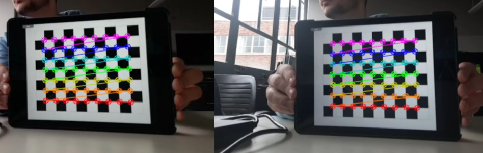
Successful matches should be as follows where all the number of the corners defined in the code are mapped and have the same color in the two images:
 |
|---|
| Fig. 3. Example of successful chessboard corner matching. |
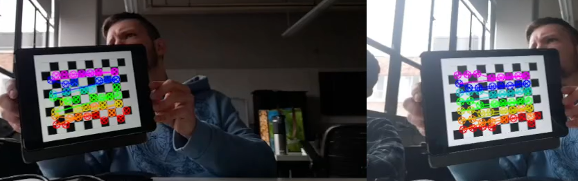
Possible issues at this stage can be that the corners are not found at all or the points are erroneously identified. If the corners are not found there is another function cv.findChessboardCornersSB() that can be used which uses a different algorithm and in our experience performed better, however ideally this should not be required.
Due to low resolution or sharp angles often the matches on the board were not the same as in the following:
 |
|---|
| Fig. 4. Example of an unsuccessful chessboard corner matching. |
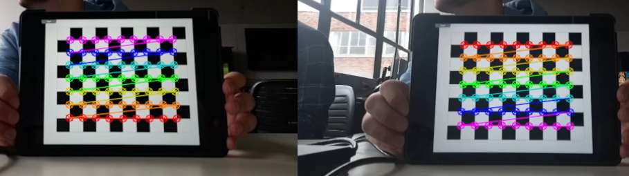
Another difficult to detect issue is when one checkerboard is detected as inverted, one can know this if the colors do not align as in the following:
 |
|---|
| Fig. 5. Unwanted inversion of color order in chessboard matching. |
It is important to remove any such images as even one such pair of images can distort the output and create errors with the rectification.
Following the identification of the points the intrinsic and extrinsic camera matrices calculation is straight forward utilizing cv.calibrateCamera() and cv.stereoCalibrate(). These matrices are then used in cv.stereoRectify() to get the mapping matrices, finally cv.initUndistortRectifyMap() is used to create the stereo map. It is useful to use the roi_L and roi_R output of stereoRectify to understand any bugs; it outputs coordinates for a rectangle for both the images that the program considers as overlapping data.
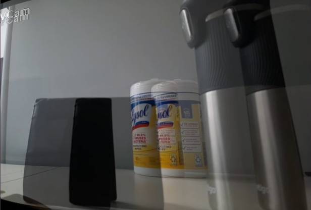
Finally, the stereo map can be used to rectify any pair of images from the camera setup using cv.remap(). A good test for successful calibration and rectification is to overlap the two images using cv.addWeighted() and check if the y axis are fully aligned as in the following image:
 |
|---|
| Fig. 6. An example of proper vertical alignment of the stereo image pair. |
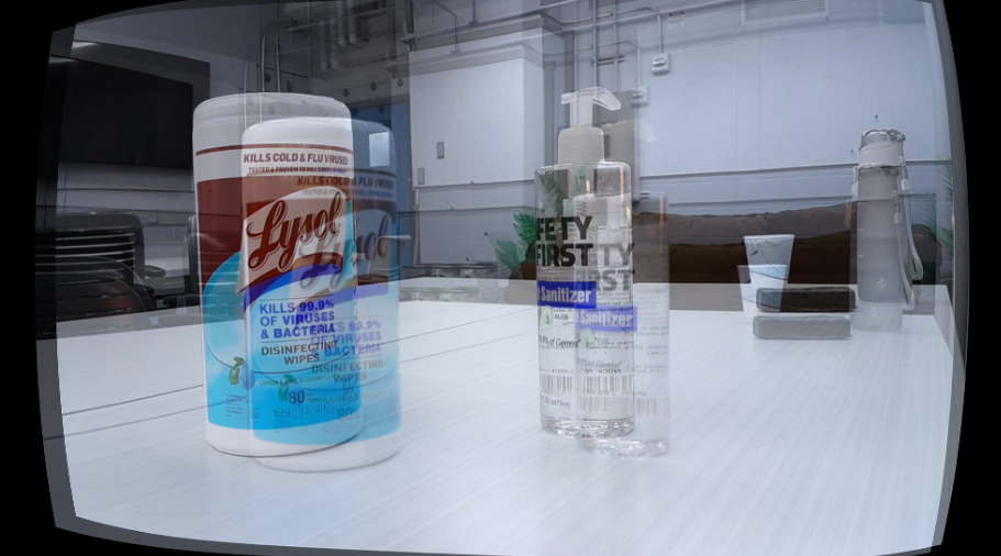
A poorly overlayed example could be:
 |
|---|
| Fig. 7. An example of poorly aligned stereo image pair. |
There are multiple issues that are possible in calibration and rectification and it is important to test at the intermediate steps utilizing the methods mentioned above.
Creating the disparity map
Once images have been rectified and are aligned the disparity map can be created using the function cv.StereoBM() or cv.StereooSGBM(). The function has multiple parameters that directly affect the output and their respective descriptions can be read here. It can be useful to create a tool to alter the parameters in real time and see the results. We altered a code to work with static images to experiment with different settings of the parameters. Below is an example of how this could be done:
block_size = 11
min_disp = -128
max_disp = 128
num_disp = max_disp - min_disp
uniquenessRatio = 5
speckleWindowSize = 200
speckleRange = 2
disp12MaxDiff = 0

matcher = cv.StereoSGBM_create(
    minDisparity=min_disp,
    numDisparities=num_disp,
    blockSize=block_size,
    uniquenessRatio=uniquenessRatio,
    speckleWindowSize=speckleWindowSize,
    speckleRange=speckleRange,
    disp12MaxDiff=disp12MaxDiff,
    P1=8 * 1 * block_size * block_size,
    P2=32 * 1 * block_size * block_size,
)

disparity = matcher.compute(imgL_rect, imgR_rect)
Post processing the disparity map
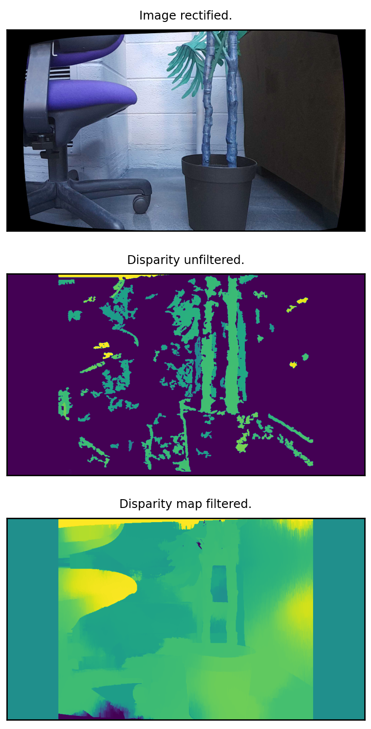
Post processing of the disparity map is an important step for achieving better results. In our experiment, the cv.ximgproc.createDisparityWLSFilter() is used. More on it can be read on the official OpenCV tutorial , as well as this Stackoverflow discussion. Our implementation uses both disparity maps - the left and right one, to create a cleaner version. The following examples show the difference between a raw disparity map and a filtered one:
 |
|---|
| Fig. 8. Comparison of raw and filtered disparity map. |
Below a sample function constructing and filtering a disparity map can be found:
def disp_filtering(imgL_rect, imgR_rect, left_matcher, lmbda=8000, sigma=1.5):
    '''
    Function filters the raw disparity map, giving a better representation.
    :param imgL_rect: left rectified image.
    :param imgR_rect: right rectified image.
    :param left_matcher: a matcher object like cv.StereoSGBM_create().
    :param lmbda: Lambda is a parameter defining the amount of regularization
    during filtering. Larger values force filtered disparity map edges to
    adhere more to source image edges. Typical value is 8000.
    :param sigma: SigmaColor is a parameter defining how sensitive the filtering
    process is to source image edges. Large values can lead to disparity leakage
    through low-contrast edges. Small values can make the filter too sensitive to
    noise and textures in the source image. Typical values range from 0.8 to 2.0.
    :returns: filtered left and right disparity maps.
    '''
    right_matcher = cv.ximgproc.createRightMatcher(left_matcher)
    wls_filter = cv.ximgproc.createDisparityWLSFilter(
        matcher_left=left_matcher)
    wls_filter.setLambda(lmbda)
    wls_filter.setSigmaColor(sigma)
    displ = left_matcher.compute(imgL_rect, imgR_rect)
    dispr = right_matcher.compute(imgR_rect, imgL_rect)
    fil_disp_left = wls_filter.filter(
        disparity_map_left=displ, left_view=imgL_rect, disparity_map_right=dispr)
    fil_disp_right = wls_filter.filter(
        disparity_map_left=displ, left_view=imgR_rect, disparity_map_right=dispr)
    return fil_disp_left, fil_disp_right
Real-time Rectification method
An alternative to the precalculated fundamental matrix that is achieved using the chessboard method, would be to calculate the fundamental matrix for each individual image based on the matches between the images. This method is easier to implement in comparison to the chessboard calibration, where you have to take a whole set of photos and calibrate over them. Here is the approximate pipeline one would use to achieve this:
- First, we need to rectify our images, to achieve vertical alignment. Instead of using a precalculated matrix for the two cameras, we rectify the images only based on the matches between them. Thus, we need to find those matches. We need to find keypoints in both images, so we could use something like
sift = cv.SIFT_create()andkp1, des1 = sift.detectAndCompute(). - Then we need to match the keypoints, using
cv.FlannBasedMatcher(index_params, search_params). - What if there are multiple matches to the same keypoints? We can use RANSAC to filter for only good matches. In our implementation, RANSAC is used internally, when the fundamental matrix is being found by
fundamental_matrix, inliers = cv.findFundamentalMat(pts1, pts2, cv.FM_RANSAC) - The fundamental matrix establishes a connection between the images, but we need to warp them somehow, to align the vertical levels of the images. We do this by
_, H1, H2 = cv.stereoRectifyUncalibrated(np.float32(pts1), np.float32(pts2), fundamental_matrix, imgSize=(w1, h1)). - The final step is to apply the transformation to both images, this can be done by using
img1_rectified = cv.warpPerspective(img1, H1, (w1, h1))
img2_rectified = cv.warpPerspective(img2, H2, (w2, h2)) - Profit! We have rectified our images, and now we can use the standard procedure to calculate the disparity.
Consider reading more on matching on the official OpenCV tutorial. We also used this great tutorial to understand this method. Also, here are a couple of functions that would do this process for you:
def find_matches(img1, img2):
    '''
    Function takes in two images and finds best matches between them.
    :param img1: first image.
    :param img2: second image.
    :returns: list with good matches, lists with coords from imgL and imgR.
    '''
    sift = cv.SIFT_create()
    kp1, des1 = sift.detectAndCompute(img1, None)
    kp2, des2 = sift.detectAndCompute(img2, None)

    FLANN_INDEX_KDTREE = 1
    index_params = dict(algorithm=FLANN_INDEX_KDTREE, trees=5)
    search_params = dict(checks=50)   # or pass empty dictionary
    flann = cv.FlannBasedMatcher(index_params, search_params)
    matches = flann.knnMatch(des1, des2, k=2)

    matchesMask = [[0, 0] for i in range(len(matches))]
    good = []
    pts1 = []
    pts2 = []

    for i, (m, n) in enumerate(matches):
        if m.distance < 0.7*n.distance:
            # Keep this keypoint pair
            matchesMask[i] = [1, 0]
            good.append(m)
            pts2.append(kp2[m.trainIdx].pt)
            pts1.append(kp1[m.queryIdx].pt)

    pts1 = np.int32(pts1)
    pts2 = np.int32(pts2)

    return good, pts1, pts2


def rectify_images(img1, img2, pts1, pts2):
    '''
    Rectification of images using the Fundamental Matrix.
    :param img1: first image to rectify.
    :param img2: second image to rectify.
    :param pts1: feature points in the first image.
    :param pts2: feature points in the second image.
    :returns: rectified images 1 and 2.
    '''
    fundamental_matrix, inliers = cv.findFundamentalMat(
        pts1, pts2, cv.FM_RANSAC)

    h1, w1 = img1.shape[:-1]
    h2, w2 = img2.shape[:-1]
    _, H1, H2 = cv.stereoRectifyUncalibrated(
        np.float32(pts1), np.float32(pts2), fundamental_matrix, imgSize=(w1, h1)
    )

    img1_rectified = cv.warpPerspective(img1, H1, (w1, h1))
    img2_rectified = cv.warpPerspective(img2, H2, (w2, h2))
    return img1_rectified, img2_rectified
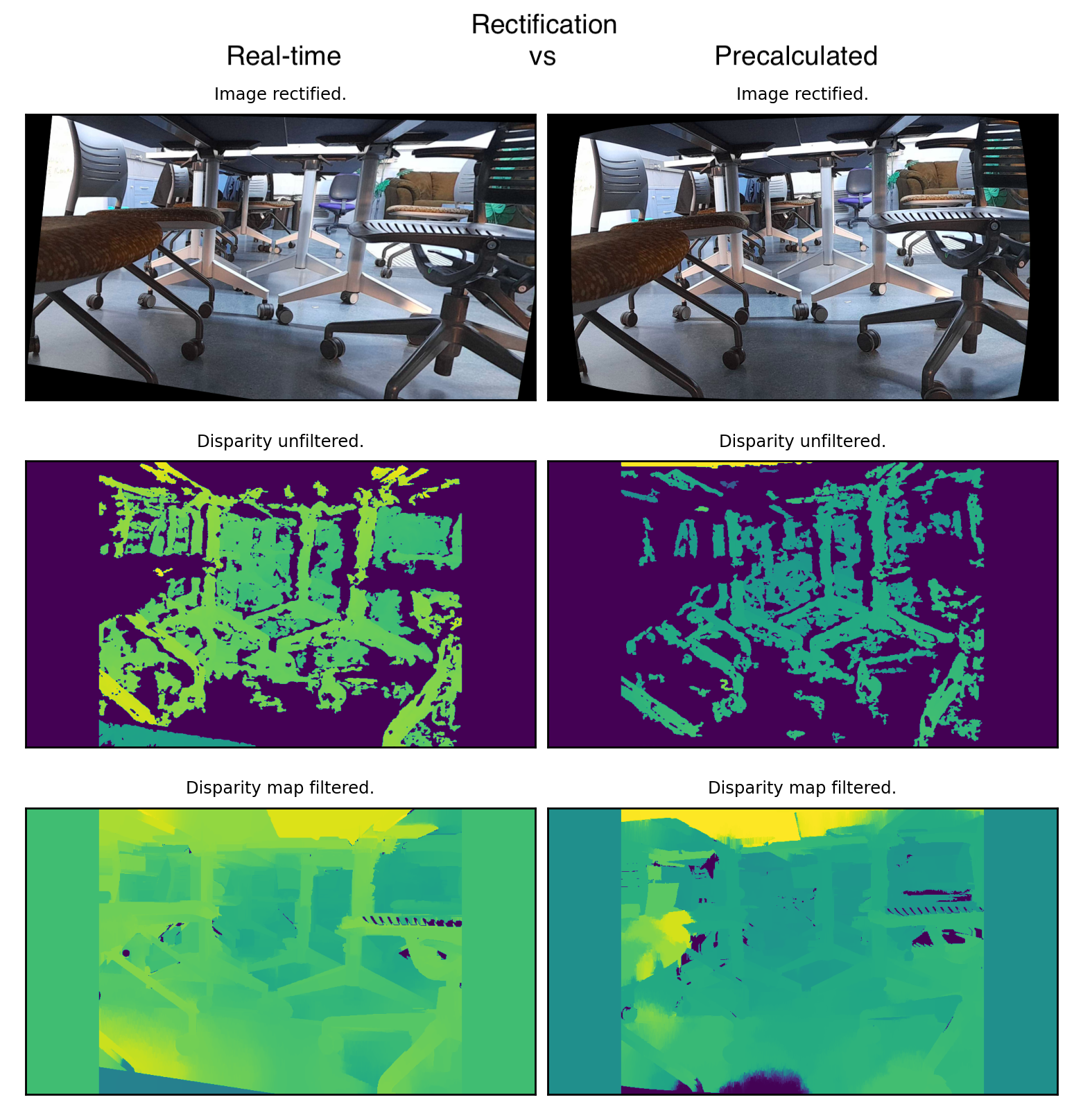
Comparison between the Real-time and Precalculated Rectification.
Comparing these two methods, we determined a number of pros and cons for both of them:
Real-time rectification Pros:
- Easier to implement than Precalculated: no need to have a stereo camera setup, or take a set of chessboard photos with it. You just need two individual images of the same scene, where feature matching can happen.
- Even though the results might be quite random (RANSAC is used), gives quite decent results.
Real-time rectification Cons:
- The results are not consistent. If you run the algorithm multiple times on the same pair of images, you get very different results sometimes, This is due to randomized feature matching. Each time you get a different fundamental matrix and different rectification.
- The algorithm can be computationally intensive, especially if one would consider doing depth maps for a video.
- The rectification transformation that is applied here can distort the image a significant amount, making the disparity map somewhat unclear.
Precalculated rectification Pros:
- The results produced are consistent throughout each image. The transformation is always the same, since the fundamental matrix is precalculated.
- Faster processing times. No need to do matching!
- Can be used for creating disparity maps for video. This is due to the consistency of the rectification as well as the processing times.
Precalculated rectification Cons:
- Complicated setup procedure, as you require a stereo camera setup. In our circumstances, rubber banding two cell phones together proved to be flimsy, so for each displacement of the cameras, ideally you have to rectify again.
- Rectification using the chessboard might be buggy, you need to pay attention to results, as discussed in the “Calibration and Rectification”.
Now, let’s compare the performance of these two methods using one set of stereo images.
 |
|---|
| Fig. 9. Comparison of Real-time and Precalculated rectification. |
As we can see, the quality is comparable, however, it depends on what the fundamental matrix is going to be for the real-time rectification method.
Results Obtained
Using this setup we managed to achieve these results. Keep in mind that applying postprocessing to your video feed can cut you some frames. Below we display 3 examples of real-time disparity maps, one of which is raw, the other two are with postprocessing.
Future Work
- The next most obvious step for future work is going from the disparity map to a depth map. For this the transformation is as follows:
$$ z=\frac{b f_{x}}{\left(u_{l}-u_{r}\right)}=\text { depth } $$ The focal length in pixels can be obtained using the following:
$$ f_{pixels} = \frac{ImageWidth * f_{mm}}{SensorWidth_{mm}} $$ Once a depth map has been created there are multiple integrations that can be done with real time robotic systems. - A 3D Printed Stand can be used to hold the cameras together with markings to have reproducible results and lower noise. Evidently our setup with a clipper and rubberbands is not very rigid if we move it around.
- This setup can also be used to train a neural network. LiDAR and radar are being commonly used to teach depth on a single image. A cheaper way could be to use a stereo setup to train an algorithm for research purposes.
References and other cool links
- Our github.
- Teslas work in depth perception.
- This guy's github has the code for calibration, triagulation, stereo calibration, stereo vision.
- Depth Maps in OpenCV - Stereo Vision with code Examples.
- Camera Calibration Theory Playlist by Shree Nayar from Columbia University.
- OpenCV depth theory.
- OpenCV documentation Depth perception using stereo camera - theory and talk of matching algorithms.
- OpenCV epipolar geometry.